Deep learning have made dramatic improvements over the last decades. Part of this is attributed to improved methods that allowed training wider and deeper neural networks. This can also be attributed to better hardware, as well as the development of techniques to use this hardware efficiently. All of this leads to neural networks that grow exponentially in size. But is continuing down this path the best avenue for success?
Deep learning models have gotten bigger and bigger. The figure below shows the accuracy of convolutional neural networks (left) and the size and number of parameters used for the Imagenet competition (right). While the accuracy is increasing and reaching impressive levels, the models get both bigger and use more and more resources. In Schwartz et al., 2020, as a result of rewarding more accuracy than efficiency, it is stated that the amount of compute have increased 300k-fold in 6 years which implies environmental costs as well as increasing the barrier to entry in the field.
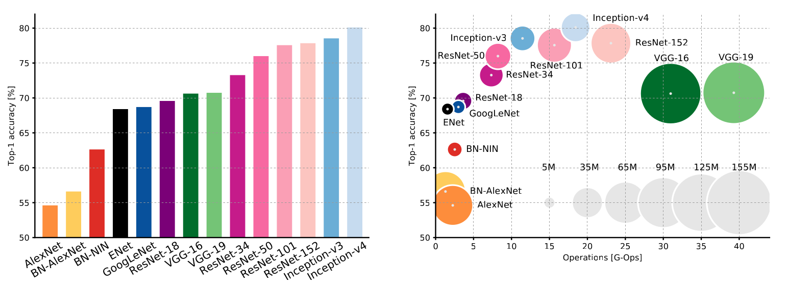
Deep learning models get better over time but also increases in size (Canziani et al., 2016).
There may be a correlation between the test loss, the number of model parameters, the amount of compute and the dataset size. The loss gets smaller as the network gets bigger, more data is processed and more compute capacity is added, which suggests a power law is at work, and that the predictions from deep learning models can only become more accurate. Does that mean neural network are bound to getting bigger? Is there an upper limit above which the rate of accuracy change slows down? In that case, changing the paradigm or finding how to get the most out of each parameter would be warranted, so that the accuracy may keep increasing without always throwing more neurons and data at the problem.
Changing the paradigm would require to change perspective and go past deep learning, which would be, giving its tremendous success, a very risky strategy which would almost certainly hamper progress on the short term. As workarounds (which do not address the underlying problem), it may be wise to reduce the models’ size during their training as a way to make them smaller. Three strategies may be employed to that end: dropout, pruning and quantization.
Dropout #
Dropout tries to make sure neurons are diverse enough inside the network, thereby maximizing the usefulness of each of them. To do that, a dropout layer is added between linear connections that randomly deactivates neurons during each forward pass through the neural network. This is done only the training (i.e. not during inference). By randomly deactivating neurons during training, one can force the network to learn with an ever-changing structure, thereby incentivzing all neurons to take part to the training. The code below shows how to use dropout in a PyTorch model definition:
|
|
A dropout that will randomly deactivate half of the neuron’s layer is defined line 5, and is used in the forward pass line 13.
Pruning #
Pruning refers to dropping connections between neurons, therefore making the model slimmer. Pruning a neural network begs the question of identifying the parts of it which should be pruned. This can be done by considering the magnitude of the neurons’ weights (because small weights may not contribute much to the overall result) or their relative importance towards the model’s output as a whole.
In PyTorch, pruning based on the weights’ magnitude may
be done with the
ln_structured
function:
|
|
The line 24 is responsible for the pruning, where the first layer of the model is half-pruned according to the l2 norm of its weights.
Quantization #
Instead of dropping neurons, one may reduce their precision (i.e. the number of bytes used to store their weights) and thus the computing power needed to make use of them. This is called quantization. There exists 3 ways to quantize a model.
Dynamic quantization #
Quantization may be done directly after the model is instantiated. In that case, the way to quantize is chosen at runtime and is done immediately.
model = NeuralNetwork(784, 100, 10)

torch.quantization.quantize_dynamic(
    model, {"l1": torch.quantization.default_dynamic_qconfig}
)
Adjusted quantization #
Quantization can be calibrated (i.e. choose the right algorithm to convert floating point numbers to less precise ones) by using the data that is supposed to go through the model. This is done on a test dataset once the model has been trained:
|
|
How the model is supposed to be quantized and de-quantized is added to the model class on line 4 and 9. Line 22 prepares the model for quantization according to the configuration of line 21. Line 24-27 create a test dataset and run it through the prepared model so that the quantization process can be adjusted. Once the calibration is done, the model is quantized to int8 at line 29.
Quantization At Training #
Quantization At Training (QAT) refers to optimizing the quantization strategy during the training of the model, which allows the model to optimize its weights while being aware of the quantization:
|
|
This looks similar to the previous example, except that the training loop is
done on the model_fp32_prepared model.
Can the trend towards bigger deep learning models be reverted? While research (e.g. Han et al., 2015; Howard et al., 2017) is pushing towards that goal, efficiency needs to be a priority.