The accuracy of a model is often criticized for not being informative enough to understand its performance trade offs. One has to turn to more powerful tools instead. Receiver Operating Characteristic (ROC) and Precision-Recall (PR) curves are standard metrics used to measure the accuracy of binary classification models and find an appropriate decision threshold. But how do they relate to each other?
What are they for? #
Often, the result of binary classification (with a positive and negative class) models is a real number ranging from 0 to 1. This number can be interpreted as a probability. Above a given threshold, the model is considered to have predicted the positive class. This threshold often defaults to 0.5. While sound, this default may not be the optimal value. Fine-tuning it can impact the balance between false positives and false negatives, which is especially useful when they don’t have the same importance. This fine-tuning can be done with ROC and PR curves, and is also useful as a performance indicator.
How to make a ROC and PR curve? #
Both curves are based on the same idea: measuring the performance of the model at different threshold values. They differ on the performance measures. The ROC curve measures both the ability of the model to correctly classify positive examples and the ability of the model to minimize false positive errors. On the other hand, the PR curve focuses exclusively on the positive class and ignore correct predictions of the negative class, making it a compelling measure for imbalanced datasets. While the two curves are different, it has however been proved that they are equivalent, because although the true negatives (correct predictions of the negative class) are not taken into account by the PR curve, it is possible to deduce it from the other measures.
Receiver Operating Characteristic (ROC) curve #
ROC curves measure the True Positive Rate (among the positive samples, how many were correctly identified as positives), and the False Positive Rate (among the negatives samples, how many were falsely identified as positive):
$$TPR = \frac {TP} {TP + FN}$$
$$FPR = \frac {FP} {FP + TN}$$
A perfect predictor would be able to maximize the TPR while minimizing the FPR.
Precision-Recall (PR) curve #
The Precision-Recall curve uses the Positive Predictive Value, precision (among the samples which the model predicted as being positive, how many were correctly classified) and the True Positive Rate (also called recall):
$$PPV = \frac {TP} {TP + FP}$$
A perfect predictor would both maximize the TPR and the PPV at the same time.
ROC and Precision-Recall curves in Python #
With scikit-learn and matplotlib (both are Free Software), creating these curves is easy.
|
|
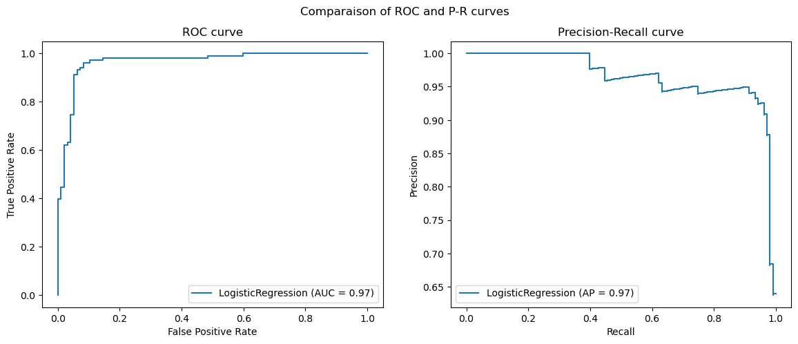
Plot of a ROC and Precision-Recall curves
Line 7-11 create a sample dataset with a binary target, split it into a training set and a testing set, and train a logistic regression model. The important lines are lines 14 and 15 which automatically compute the performance measures at different threshold values.
How to read the curves? #
Both curves offer two useful information: how to choose the positive class prediction threshold and what is the overall performance of the classification model. The former is determined by selecting the threshold which yield the best tradeoff, in adequation with the prediction task and operational needs. The latter is done by measuring the area under the curves which informs about how good the model is, because by measuring the area under the curves, one computes the overall probability that a sample from the negative class has a lower probability than a sample from the positive class.
With scikit-learn, the values can be computed either by using the roc_auc attribute of the object returned by plot_roc_curve() or by calling roc_auc_score() directly for ROC curves and by using the average_precision attribute of the object returned by plot_precision_recall_curve() or by calling average_precision_score() directly for PR curves.