Wanting to brush up my PyTorch skills, I’ve started to follow this tutorial. It explains how to create a deep learning model able to predict the origin of a name. At the end of the tutorial, there’s an invitation to try to improve the model. Which I did. Note that the point of the tutorial is not to create the most performant model but rather to demonstrate and explain PyTorch’s capabilities. Here’s a comparison between the model described in the tutorial and the one I’ve built.
Use an advanced gradient descent algorithm to optimize the network’s weights #
The code in the tutorial updates the parameters manually. Although this gets the job done, there are more efficient options, so I implemented one of them by using an optimizer.
Add this line before the train() function to define the Adam optimizer. We add L2 regularization (Try to minimize the sum of squared weights as well as the loss) with a $\lambda$ of 2e-5.
optimizer = torch.optim.Adam(rnn.parameters(), lr=learning_rate, weight_decay=2e-5)Then modify train() so it looks like this:
|
|
The optimizer.step() line updates all the model’s parameters according to
their gradients (computed by loss.backward()). The optimizer.zero_grad()
line zero out the gradients. This is mandatory because otherwise PyTorch
accumulates the gradients during the training loop.
This approach is better than the one used in the tutorial because it makes the network learn much faster and circumvent the exploding gradients problem by taking into account the general error trend when updating the parameters. Also, it is less error-prone than managing the parameters by hand as everything is handled automatically.
From a RNN to a GRU-based network #
RNNs have the perfect architecture to deal with ordered sequences. That’s why they are quite good at language modeling. The structure is simple, though. The current input and the previous state are multiplied or concatenated together. This means there’s no control of whether we should use the previous state. That’s a lack of control, Also, RNNs suffers from the vanishing gradient problem. Gated Recurrent units (GRUs) are much less sensitive to it and offer a fine-grained control over the information to keep or discard at each pass.
As an input to the GRU, I use an embedding layer, which turns each letter into a vector of 256 dimensions. This allows the model to have a rich representation of the letters.
Model definition #
The model is very different from the one in the tutorial. The full code is below:
|
|
The first layer (defined line 5 and used line 13) is the embedding layer. Given a letter ID, it outputs a vector. The vectors are initialized with Xavier’s formula, meaning that the initial variance of the vector will be $\frac{2}{f_{an\_in} + f_{an\_out}}$. $f_{an\_in}$ and $f_{an\_out}$ are the number of inputs and the number of outputs, respectively.
Right after the embedding layer, we use the GRU (defined line 7 and used line
14). As the GRU’s input needs to be in the format (seq length, batch size,
input size), we use embedding.view(len(input), 1, -1) to add the batch size
dimension. For example, for a name with 6 characters, the embedding layer
output will be in the format (6, 256). We turn it into (6, 1, 256) so that
the GRU knows there’s only one batch, because we send only one name at a time.
As we don’t provide a hidden state to the GRU, it is initialized to zeros.
Last but not least, we grab the final GRU output and map it to the number of classes (the possible name’s origin) line 15. Softmax (line 17) is used to get a probability distribution.
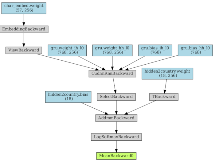
Here is how the model’s graph looks like:
Input and training loop changes #
This models requires several changes to randomTrainingExample() and
train(). First, I modify the randomTrainingExample() function so that the
input is integer-encoded instead of being one-hot encoded like in the tutorial.
The embedding layer can thus convert the input to the vectorized representation:
|
|
Next, the train() function is updated so that the entire name is passed to the
network all at once, instead of sending one letter at a time like in the
tutorial:
|
|
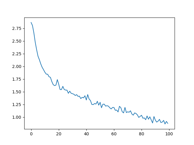
Results #
Loss #
The loos is much better than the one from the tutorial:
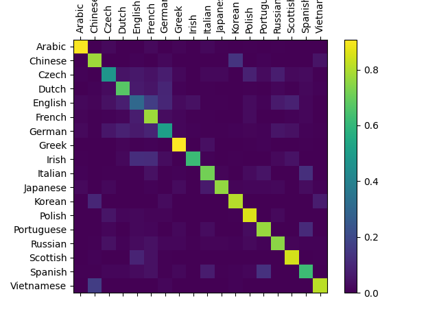
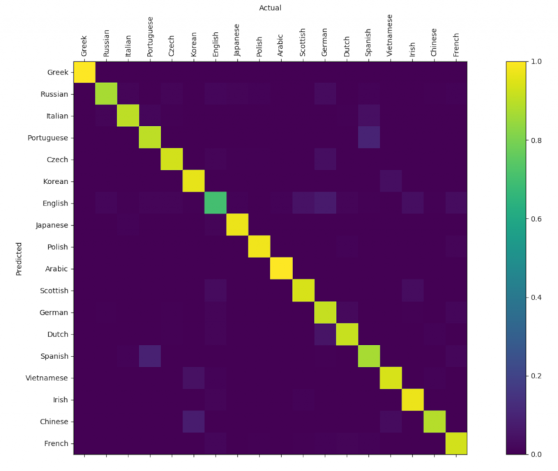
Confusion matrix #
Here is the confusion matrix showing the classification accuracy. We can see that it is much better that the one from the tutorial.
Conclusion #
By making the model more sophisticated, we increased its accuracy a lot. The model architecture presented here is suitable for a lot of text classification tasks, although entire sentences or paragraphs classification would benefit from a word embedding rather than the character embedding shown here.