SymPy is a lightweight symbolic mathematics library for Python under the 3-clause BSD license that can be used either as a library or in an interactive environment. It features symbolic expressions, solving equations, plotting and much more!
Creating and using functions #
Creating a function is as simple as using variables and putting them into a mathematical expression:
|
|
Line 1 imports the x and y
Symbols
from the abc collection of Symbols, line 3 creates the f function which is
$2x^2 + 3y + 10$, and line 4 evaluates f with values 3 and 5 for x and y,
respectively.
SymPy exports a large list of mathematical functions for more complex expressions such logarithm, exponential, etc., and is able to analyze the fucntion’s characteristics over arbitrary intervals:
|
|
Plotting #
SymPy is able to easily plot functions on a given interval:
|
|
Line 1 imports the
plot()
function, line 3 creates the f Function object from the sigmoid
expression $\frac{1}{1+\exp^{-x}}$, line 4 plots f and its derivative between
-5 and 5, lines 5-6 set the legends labels and lines 7 shows the created plot:
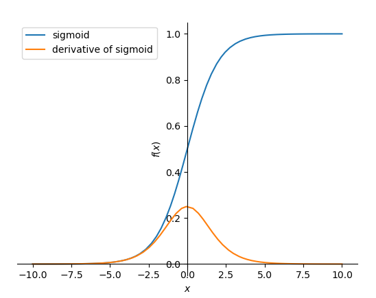
Sigmoid and its derivative.
In a few lines of code, the library allows one to create a mathematical function, do operations on it like computing its derivative and plot the result. Moreover, as SymPy uses Matplotlib under the hood by default, the plots are modifiable using the Matplotlib API.
SymPy also supports 3D plots with the
plot3d()
function which helps understanding the relationship between two variables and an
outcome. The following code computes the energy of the recoiling electron after
Compton scattering depending on the initial photon energy and the scattering
angle (in degrees) using the Compton scattering
formula : $$\beta = \arccos
\left(1 - \frac{Ee * 511}{E0 * (E0 - Ee)}\right) * \frac{180}{3.14159}$$
|
|
Line 1 imports the plot3d function, line 3 creates the E0 (the initial
photon energy) and theta custom variables1, line 4 defines the beta
function which depends on the E0 and Ee variables, line 6 does the
plotting and defines the axes intervals, line 7 sets the axes’ labels and line 8
displays the following figure:
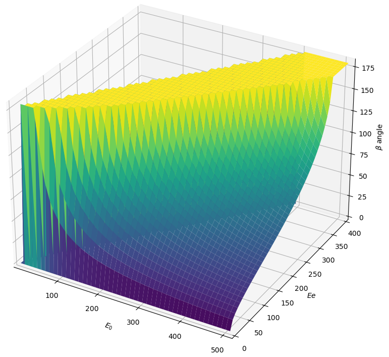
Compton angle depending on E0 and Ee.
Solving equations #
SymPy also has an equation solver for algebraic equations and equations systems: SymPy considers the equations strings to be equal to zero for ease of use.
|
|
The equation solvers also works for boolean logic, where SymPy tells what should be the truth values of the variables to satisfy a boolean expression:
|
|
An unsatisfiable expression yields False.
Geometry #
SymPy also features a geometry module allowing to perform geometric operations such as Points, Segments and Polygons. It’s
|
|
Line 1 imports classes from the geometry module, Line 2 import the SymPy plotting backends library, which contains additional plotting features needed to plot geometric objects, line 3 and 4 create a polygon and a segment, respectively, line 6 plots the figure and line 7 returns the intersection points of the polygon and the segment. Line 6 produces the following figure:
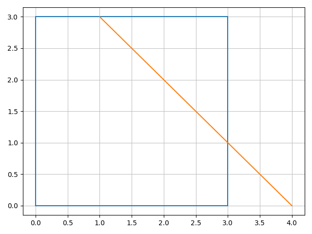
Compton angle depending on E0 and Ee.
The SymPy library is thus easy to use and suitable for various applications. Because it’s Free Software, anyone can use, share, study and improve it for whatever purpose, just like mathematics.
-
We could use the
xandyvariables here but having custom variables names makes reading the code easier. ↩︎